TL;DR
I recently built a RAG pipeline from scratch over Weaviate’s documentation. Ten iterations, twelve test queries, and a lot of wrong turns later, here’s what I learned:
- Data preparation is a significant piece of work, and almost certainly a bigger job than you think it will be.
- You need a systematic evaluation framework from day one — fixed test queries, benchmark answers, and a way to distinguish retrieval failures from generation failures.
- A bigger embedding model doesn’t automatically mean better results — bge-large performed worse than bge-base in my tests.
- Chunking strategy matters enormously, but there’s a ceiling to what chunking alone can achieve. Reranking broke through where chunking couldn’t.
- Some queries resist every optimization you throw at them until you reach for a fundamentally different technique.
Introduction
I’ve recently had conversations with several companies and AI vendors supplying technology to enterprises and it seems that RAG is pretty much top of mind for everyone. To get an insight of what’s involved in a RAG project I decided to try and build one from scratch.
The first thing I needed to decide is what data would I be building this RAG system over. I’d recently started playing with Weaviate (a popular vector database) for RAG and their documentation is open source on github, so ideal. I’d build a RAG system over their documentation, which I could then use myself.
I took a look at their documentation repo and saw it’s mostly md and mdx files. So the high level plan was:
- Clone the docs repository
- Parse all the markdown doc files
- Chunk them using some strategy
- Embed the chunks
- Load into weaviate
- Ask some questions
- Judge the answers
On closer inspection of the documents, I found that actually many of the MDX files reference code snippets from other files, so I’d need some way of following these references and render out a complete document which would then be chunked. Straightforward enough, or so I thought. What I found though was many edge cases that needed to be addressed. What I expected to be an hour job ended up taking several hours to work through. There comes a point where you have to draw a line under it and say parsing is good enough. I’d learned lesson 1:
Data preparation is a significant piece of work, and almost certainly a bigger job than you think it will be.
Once the full set of complete rendered documents was prepared, I needed to chunk them. And in the world of chunking, there are more than a dozen categories of chunking strategies that I’m aware of1 and I’m not sure if this is an exhaustive list either, and, within each category, there are different parameters you can choose and tune. Where to start, and what to tune? I decided the best step was to pick the simplest, review the results, and take it from there. So I went with Fixed-size chunking, 500 chars, no overlap. The simplest place to start.
Next, embedding the chunks. Weaviate has an API to embed directly, but I was
planning to use
Embedded Weaviate
and it seemed simpler for me to embed the chunks outside of weaviate, using
Sentence Transformers
and then just pass these embeddings to Weaviate. GPU offload on MacBook
(MLX) is as simple as
device="mps" with Sentence Transformers so that was a good way to speed things
up.
Once this was done, I needed to test some queries. A parameter you need to choose is top-k, that is, the number of results you want back. If you choose a larger top-k value you’ll get back a larger number of results back. There is a trade-off, more results may mean you’re more likely to get the chunk you need with the useful information the user is looking for, but you’ll probably also get more irrelevant results, that may pollute context with noise that could degrade final results, and it’ll certainly cost more because the input token count will be higher.
At this point I noticed, I’m doing a lot just choosing methods and values, often at random, at best, as an educated guess. That’s something I’ll do more as I go on, and something that seems to be part of building a RAG system in general. There are so many options, and datasets vary, and expected queries vary, there isn’t really a one size fits all, so it’s often about experimenting to find what works best for your use case. So I decided I needed to do better than just randomly type in queries and look at results — I needed to be systematic about this. I’d learned lesson 2:
You need a systematic evaluation framework from day one — fixed test queries, benchmark answers, and a way to distinguish retrieval failures from generation failures.
Testing methodology
There are a number of items you’ll record as part of your testing methodology, tracking inputs and outputs. First off:
Test queries
These are the set of questions you’ll use each time, and when you change something, a parameter or model, you’ll run the same queries again and compare the results. I landed on 4 test queries.
- What is the latest Weaviate version?
- How do I install Weaviate?
- What is the Weaviate license?
- What is weaviate embedded mode?
Chunks returned
For each query, what chunks were returned. This is needed because when your answer isn’t “good enough” you’ll need to know: is the issue with generation (the LLM was given the right context but didn’t extract the salient information correctly) or with retrieval (the LLM never got the right context in the first place)? This distinction turns out to be one of the most important things to track.
Things being changed
In this first step, I’d try several top-k values and compare the results.
Short document bias
I noticed that for a couple of queries, 2-3 of the top 5 chunks returned were very short — sometimes just a few words. These were “runt” chunks created when a document’s length doesn’t divide evenly into 500-character blocks, leaving a tiny leftover fragment at the end.
This turns out to be a well-known problem in dense retrieval: short document bias. When you embed a short chunk — say, one that just contains the word “Weaviate” — its embedding vector sits very close to queries that mention Weaviate, because there’s almost no other semantic content to dilute the match. A 500-character chunk containing a detailed explanation of Weaviate’s licensing actually scores lower than the single-word chunk, because its embedding has to represent a broader range of concepts. The result is that these runt chunks consistently outrank the chunks that contain the information you actually need.
I analysed the chunk size distribution across all 10,327 chunks:
- 158 chunks (1.5%) were under 200 characters after stripping whitespace
- 79 of those were under 100 characters
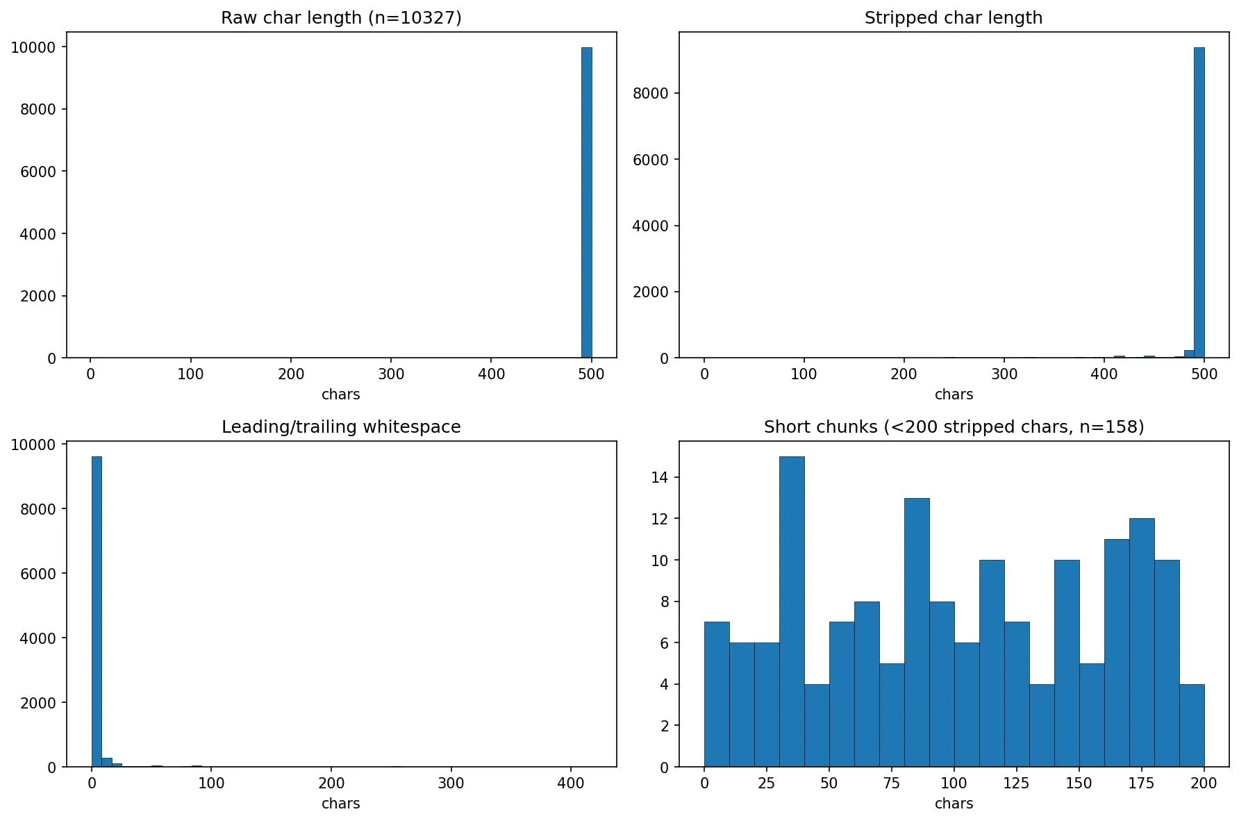
Only 1.5% of chunks were runts, but they were disproportionately appearing in the top results. The fix was simple: append the final runt chunk to the penultimate chunk, so no chunk falls below the 500-character minimum.
This was a small fix, but it illustrates a broader point: dense retrieval has failure modes that aren’t obvious until you look at what’s actually being returned. If I’d only looked at the final LLM-generated answers without inspecting the retrieved chunks, I might never have spotted this.
At this point the obvious question came: what is a good answer? And is what I have returned, good? I discovered I’d started with the harder test — an arbitrary set of queries. The more methodical way of doing this would be to select a chunk, craft a query where the answer is in that chunk, and then test to see if the chunk is returned. But I’d started down this path, and since I’d be exploring chunking strategies next, having queries that genuinely tested the system felt more representative of real use. I think in a production system you’ll need to work with people who have detailed knowledge of the documentation, or you’ll need to read it all, to gain a deep understanding of the content, so you can judge, for any given answer, if it’s “good enough”. I fortunately had a cheat code here. These documents are hosted on docs.weaviate.io and it has a built-in AI Search feature. Given that it’s Weaviate, one can assume it’s a fairly sophisticated RAG system, so the answers are likely to be pretty good. So I ran each query through this and documented the answer. These would act as my benchmark answers.
The next question to answer was, how to actually “measure” answers. How could I compare one set of answers against the benchmark?
LLM-as-a-Judge
LLM-as-a-judge is a technique where you feed the answer back into an LLM and ask it to judge the response. Of course to do that it needs something to judge it on or against. Luckily we have our benchmark answers. I ended up doing a couple of iterations on this. The first iteration sent the benchmark answer and our answer and asked it to score on a scale of 1 to 5. A description of each level was provided, from 0 — Contains none of the information found in the benchmark answer, to 5 — Contains all the information in the benchmark answer. However I found this to be a bit flaky and still a little subjective, so I ended up with the following process. A first LLM pass would extract facts and information from the benchmark answer, then for each test run, the judge would review how many of these facts or pieces of information were present in the test case answer. I found this to be a more reliable judge. I also set the temperature to 0 to try and maximise consistency and minimise hallucinations.
Test 1
500-char-no-runt chunking strategy, vary top-k using values of 5, 10, and 15.
The numbers in parentheses next to each query represent the number of key facts extracted from the benchmark answer — so “Install (13)” means the benchmark answer contained 13 distinct pieces of information.
| k | Version (3) | Install (13) | License (2) | Embedded (10) | Total |
|---|---|---|---|---|---|
| 5 | 0/3 | 2/13 | 2/2 | 5/10 | 9/28 |
| 10 | 0/3 | 2/13 | 2/2 | 6/10 | 10/28 |
| 15 | 0/3 | 2/13 | 2/2 | 5/10 | 9/28 |
These results were not great. For the Version query, I wasn’t getting any useful information back. Install returned a couple of good points, but the benchmark answer had many more. I was able to return all the relevant information about licensing, and about half of what is expected for information about Embedded Weaviate. Interestingly, increasing top-k didn’t do much to help and because I’d been recording the chunks returned, I could see that it was a retrieval issue, not a generation issue. The data was not in the chunks in the first place.
I decided to try a different, much more coarse chunking strategy — document-level chunking. I’d embed each document as is.
Test 2
Document-level chunking strategy, vary top-k using values of 5, 10, and 15
| k | Version (3) | Install (13) | License (2) | Embedded (10) | Total |
|---|---|---|---|---|---|
| 5 | 2/3 | 5/13 | 0/2 | 7/10 | 14/28 |
| 10 | 2/3 | 5/13 | 0/2 | 7/10 | 14/28 |
| 15 | 2/3 | 6/13 | 0/2 | 7/10 | 15/28 |
Here we see some improvements across 3/4 queries, but a degradation in performance for the question about licensing. Again, looking at the chunks returned, the missing information is all an issue of retrieval, not generation. The missing information is not in the retrieved chunks. Increasing K also doesn’t make much difference.
Next I tried a chunking strategy in the middle of these two extremes: structural chunking. Given the documents are markdown, sections are relatively simple to extract, though it requires a few extra steps in the chunking strategy.
The markdown-sections strategy splits a document at header boundaries (h1–h6), then builds a breadcrumb trail from the header hierarchy (e.g. “Installation > Docker > Setup”). Each chunk is prefixed with the document title and its breadcrumb, giving the embedding model semantic context about where the content sits in the doc. If any section exceeds 2000 characters, it’s split further at paragraph boundaries to keep chunks manageable. Empty sections (headers with no body) are dropped.
Test 3
Markdown structure chunking, vary top-k using values of 5, 10, and 15
| k | Version (3) | Install (13) | License (2) | Embedded (10) | Total |
|---|---|---|---|---|---|
| 5 | 0/3 | 1/13 | 2/2 | 6/10 | 9/28 |
| 10 | 2/3 | 1/13 | 2/2 | 5/10 | 10/28 |
| 15 | 2/3 | 5/13 | 2/2 | 7/10 | 16/28 |
This strategy performs well across all of the queries, not perfect but we can see we’re moving in the right direction.
I was curious how much of a difference the added breadcrumbs made. It turns out a lot.
Test 4
Markdown structure without breadcrumbs chunking, vary top-k using values of 5, 10, and 15
| k | Version (3) | Install (13) | License (2) | Embedded (10) | Total |
|---|---|---|---|---|---|
| 5 | 1/3 | 1/13 | 2/2 | 0/10 | 4/28 |
| 10 | 1/3 | 1/13 | 2/2 | 5/10 | 9/28 |
| 15 | 1/3 | 2/13 | 2/2 | 5/10 | 10/28 |
The explanation for this is that when prepending something like “Installation > Docker > Setup” to the chunk, it gives the embedding model more to work with when matching it to a query like “How do I install Weaviate?”
So at this point we’d made good progress, from 10/28 facts returned to 16/28. But looking at the per-query breakdown, one query stood out: Install. It scored 2/13, then 5/13, then 1/13, then 1/13 across the first four tests. No chunking strategy was consistently helping it. The installation information in Weaviate’s docs is spread across multiple pages and sections — Docker setup, Kubernetes, embedded mode, cloud — and no single chunk captures enough of it. This would become a recurring theme: some queries simply resist better chunking and need a fundamentally different retrieval approach.
We had a few different directions we could go in next:
- Try a different embedding model
- Try adding a reranker
- Try retrieval augmentation and hybrid search
- Try query transformation.
We’ll dive into these later, but first. I came across Rethinking Chunk Size for Long-Document Retrieval: A Multi-Dataset Analysis (Bhat et al., 2025). In this paper the authors show that chunking effectiveness is model-dependent and not just a function of the content. Their encoder-based model (Snowflake, 8K context window) consistently outperformed at smaller chunk sizes. Since bge-base-en-v1.5 is also an encoder-based model with a hard 512-token ceiling, it falls squarely into the Snowflake camp and is architecturally biased toward shorter, more focused chunks where the embedding doesn’t have to compress too much semantic content into a single vector. So I took a look at the chunk size distribution.
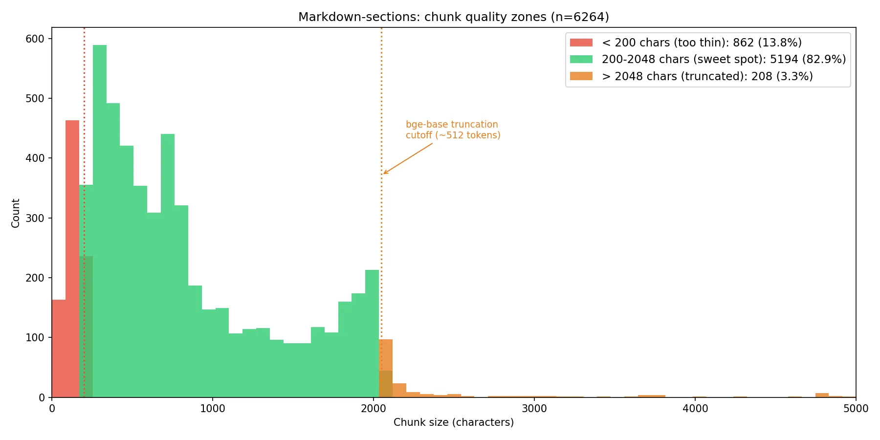
We can see from this analysis that we have a substantial right tail. Everything above roughly 2,048 characters (~512 tokens) is getting silently truncated by the model. We also have a lot of very short chunks under ~200 chars (~50 tokens). These are probably section headers, single-line config snippets, or stub sections. They’ll produce embeddings that may match too promiscuously or not at all.
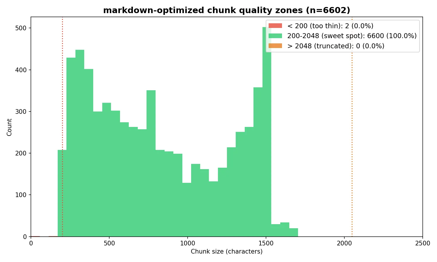
The solution was to create an optimized version of the markdown chunking strategy. This strategy splits documents at markdown header boundaries (just like markdown-sections), then applies three additional optimizations. First, it computes a per-section body budget by subtracting the breadcrumb prefix length from the 1,500-character target, so the final embedded text — including the “Document Title > Section > Subsection” prefix — stays within bge-base’s 512-token (~2,048 character) context window. Sections exceeding the budget are split at paragraph boundaries, with a word-boundary hard split as a fallback for monolithic paragraphs like large code blocks. Second, adjacent chunks under 200 characters are merged forward into their neighbor (with a backward merge for trailing runts) to eliminate thin chunks that produce low-quality embeddings. Third, each child chunk stores a reference to its full parent section text; at query time, the retriever matches against focused child embeddings but passes the richer parent context to the LLM, deduplicating parents so the model sees each section at most once.
Test 5
Markdown structure optimized chunking, vary top-k using values of 5, 10, and 15
| k | Version (3) | Install (13) | License (2) | Embedded (10) | Total |
|---|---|---|---|---|---|
| 5 | 2/3 | 0/13 | 2/2 | 7/10 | 11/28 |
| 10 | 2/3 | 1/13 | 2/2 | 7/10 | 12/28 |
| 15 | 2/3 | 5/13 | 2/2 | 7/10 | 16/28 |
The fixes improved k=5 and k=10 notably — Version query jumped from 0/3 to 2/3 at k=5, and the Embedded query from 6/10 to 7/10. It seems we have a ceiling of 16/28 when k is 15.
Next I tried a larger model. bge-large-en-v1.5 is also 512 tokens max. Same BERT-based encoder architecture, same truncation behavior. The only difference is 1024 dimensions instead of 768.
Test 6
Markdown structure optimized chunking, this time using bge-large and vary top-k using values of 5, 10, and 15
| k | Version (3) | Install (13) | License (2) | Embedded (10) | Total |
|---|---|---|---|---|---|
| 5 | 2/3 | 0/13 | 2/2 | 6/10 | 10/28 |
| 10 | 2/3 | 0/13 | 2/2 | 7/10 | 11/28 |
| 15 | 2/3 | 1/13 | 2/2 | 7/10 | 12/28 |
Interestingly these results are worse for every value of k. I’d learned lesson 3:
A bigger embedding model doesn’t automatically mean better results — bge-large performed worse than bge-base across the board.
Next we tried a reranker, back using bge-base. The purpose of a reranker is to cast the net wider with a larger initial retrieval, then whittle down to a smaller set by passing results through a cross-encoder. Cross-encoders are slower than bi-encoders but can more accurately rank the relevance of each chunk to the query, because they process the query and chunk together rather than comparing pre-computed embeddings. We tested several different combinations.
Test 7
Markdown structure optimized chunking, bge-base, varying retrieval-k and rerank-to-k
| retrieve | rerank to | Version (3) | Install (13) | License (2) | Embedded (10) | Total |
|---|---|---|---|---|---|---|
| 50 | 10 | 2/3 | 5/13 | 2/2 | 6/10 | 15/28 |
| 100 | 15 | 2/3 | 6/13 | 2/2 | 6/10 | 16/28 |
| 200 | 15 | 2/3 | 7/13 | 2/2 | 6/10 | 17/28 |
| 250 | 10 | 2/3 | 6/13 | 2/2 | 6/10 | 16/28 |
| 250 | 20 | 2/3 | 9/13 | 2/2 | 6/10 | 19/28 |
| 300 | 20 | 2/3 | 7/13 | 2/2 | 6/10 | 17/28 |
Retrieve 250, rerank to 20 was the sweet spot, hitting 19/28 — our best result yet.
The Install query is the headline here. It jumped from 0/13 in Test 5 to 9/13 — the reranker finally cracked the query that had resisted every chunking optimisation. The broader initial retrieval (250 chunks) pulled in installation-related content that wasn’t making the top 15 in pure semantic search, and the cross-encoder was able to identify which of those 250 were genuinely relevant.
Two things worth noting. First, retrieve 300 performed worse than retrieve 250. More candidates isn’t always better — the additional noise can dilute the reranker’s signal. Second, the Embedded query actually regressed from 7/10 (Tests 2, 5) to 6/10 across every reranker configuration. The reranker helped Install significantly but consistently hurt Embedded. This trade-off is important: in a production system, optimising for one query type can degrade another, and you’d need to monitor for this.
The reranker result taught me two more lessons. Lesson 4:
Chunking strategy matters enormously, but there’s a ceiling to what chunking alone can achieve. Reranking broke through where chunking couldn’t.
And lesson 5, courtesy of the Install query:
Some queries resist every optimisation you throw at them until you reach for a fundamentally different technique.
The Install query scored 2/13, 5/13, 1/13, 1/13, 0/13 across five chunking tests. Only the reranker cracked it — jumping to 9/13 in a single step. If I’d kept tuning chunk sizes and overlap, I’d still be stuck at zero.
Hybrid search is a common technique to improve retrieval by combining semantic search results with keyword (BM25) search results before passing them to the reranker. Before running the test, I went digging through the data manually. As well as getting the benchmark answers from docs.weaviate.io, the responses also contained the source documents the answers were drawn from. Since I’d been logging the chunks returned for each call, I could determine which documents were missing from the retrieval. I did a manual keyword search over those missing documents to see if BM25 would help surface them, but it didn’t look promising — our queries are short (5–8 words) with few distinctive keywords, and the missing chunks didn’t contain those words.
Test 8
Markdown structure optimized chunking, bge-base, retrieval-k 250 with hybrid search (75% semantic and 50/50), reranking top-k 20
| Search | Version (3) | Install (13) | License (2) | Embedded (10) | Total |
|---|---|---|---|---|---|
| vector-only | 2/3 | 9/13 | 2/2 | 6/10 | 19/28 |
| hybrid α=0.75 | 2/3 | 8/13 | 2/2 | 6/10 | 18/28 |
| hybrid α=0.5 | 2/3 | 6/13 | 2/2 | 6/10 | 16/28 |
As expected, hybrid search didn’t improve results — in fact, the more weight given to keyword matching, the worse performance got. The likely explanation: with short, general queries like “How do I install Weaviate?”, keyword matching adds noise rather than signal. The word “install” appears in hundreds of chunks across the corpus, most of which aren’t relevant to the specific installation information needed. Hybrid search would likely help more with longer, more specific queries containing distinctive technical terms.
HyDE (Hypothetical Document Embedding) is a query transformation technique introduced by Gao et al. in Precise Zero-Shot Dense Retrieval without Relevance Labels. The idea is to pass the original query to an LLM and ask it to generate a completely hypothetical response. It doesn’t need to be grounded in any truth — the answer can be entirely made up. This hypothetical document is then embedded and used to search across the chunks, replacing the original query embedding. The retrieved chunks and the original query are then sent to the LLM for the final answer. The technique is shown to improve retrieval relevance by bridging the semantic gap between short queries and longer document passages. The hypothetical document captures relevance patterns even if the facts are wrong, and the encoder’s dense bottleneck filters out the hallucinations by grounding to real documents in the corpus.
Test 9
Markdown structure optimized chunking, bge-base, HyDE step, retrieval-k 250, reranking top-k 20
| Version (3) | Install (13) | License (2) | Embedded (10) | Total |
|---|---|---|---|---|
| 2/3 | 9/13 | 2/2 | 6/10 | 19/28 |
The total was identical to the baseline — 19/28 with or without HyDE. However, looking at the per-query breakdown in later tests with more queries would reveal that HyDE doesn’t produce the same results, it produces different results that happen to sum to the same total. It helps some query types and hurts others, reshuffling which retrieval errors occur rather than reducing them overall. For a production system, this means HyDE might be worth enabling selectively for certain query patterns rather than as a blanket improvement.
At this point I wanted a broader set of test queries to validate these findings. I used Claude Code to script the data exploration — writing analysis scripts to narrow down where missing information was and what we could do to improve results. I expanded the test set from 4 to 12 queries. The Weaviate docs site also has an MCP interface, which made generating benchmark answers for the new queries straightforward — I could ask Claude Code to query docs.weaviate.io directly and add the results to the evaluation spreadsheet.
Test 10
Markdown structure optimized chunking, expanded query set, bge-base, with and without HyDE step, retrieval-k 250, reranking top-k 5
| Config | Version (3) | Install (12) | License (2) | Embedded (10) | HNSW (18) | Multi-tenant (17) | Backups (16) | Hybrid (19) | RBAC (16) | Replication (14) | RAG (14) | Filtering (17) | Total |
|---|---|---|---|---|---|---|---|---|---|---|---|---|---|
| baseline | 2/3 | 9/12 | 2/2 | 6/10 | 15/18 | 12/17 | 13/16 | 11/19 | 14/16 | 12/14 | 9/14 | 13/17 | 118/158 (74.7%) |
| HyDE | 2/3 | 10/12 | 2/2 | 6/10 | 13/18 | 13/17 | 13/16 | 11/19 | 13/16 | 13/14 | 10/14 | 12/17 | 118/158 (74.7%) |
The expanded test set confirmed the pattern: 74.7% fact coverage against a sophisticated benchmark RAG system, using structural chunking, a reranker, and a relatively small embedding model. With and without HyDE, the total was identical at 118/158 — but the per-query scores shuffled around (Install +1, HNSW -2, Multi-tenant +1, RBAC -1, Replication +1, RAG +1, Filtering -1), confirming that HyDE changes the pattern of retrieval errors rather than reducing them.
One thing to note: Install dropped from 13 to 12 key benchmark facts in this run. The LLM judge extracted slightly different facts from the MCP-sourced benchmark answer this time around. Previously, facts had been extracted once, cached, and reused for each test run. This time, due to the new queries, we did a fresh fact extraction pass. LLMs are non-deterministic even with temperature set to 0 — so in a production evaluation system, it may be worth running the judge multiple times and taking an average or maximum value.
What I’d tell an enterprise team starting a RAG project
After ten iterations and a lot of wrong turns, here’s what I’d want someone to know before they start.
Data preparation will take longer than you think, and it’s the most important step you’ll do. I expected an hour of parsing work and spent the better part of two days building an import graph resolver to handle Docusaurus’s nested MDX imports. Every documentation system has its own version of this problem — Confluence has its storage format with custom macros, Jira uses Atlassian Document Format, SharePoint has its own idiosyncrasies. Whoever tells you “just point the RAG system at your docs” hasn’t done it with real enterprise content.
Build your evaluation framework before you build your pipeline. I did this in the wrong order and wasted time running ad hoc queries that told me nothing useful. Fixed test queries, benchmark answers, and a systematic way to score results — ideally with LLM-as-judge using fact extraction rather than subjective scoring — should be the first thing you set up, not an afterthought.
Chunking strategy matters, but there’s a ceiling. I went from 9/28 with naive fixed-size chunks to 16/28 with optimised structural chunking — a significant improvement. But no amount of chunking optimisation could push past that ceiling. The breakthrough came from a fundamentally different technique: reranking. The lesson is that when you’re stuck, the answer is usually in a different part of the pipeline, not more tuning of the same component.
Bigger models aren’t automatically better. bge-large performed worse than bge-base on every metric I tested. The likely explanation is that for this corpus and these queries, the additional embedding dimensions added noise without adding useful discriminative signal. Always test — don’t assume that the larger or newer model is the right choice.
Some queries are fundamentally harder than others, and you need to know which ones you have. The Install query resisted five iterations of chunking improvements and only broke through with a reranker. If your users are asking questions that require synthesising information scattered across many documents, no amount of single-retrieval optimisation will solve the problem. That’s where agentic approaches — multi-step retrieval, query decomposition, iterative search — become necessary. That’s the subject of my next post.
Negative results are results. Hybrid search didn’t help. HyDE didn’t improve the total. bge-large was worse. These findings are just as valuable as the improvements, because they tell you where not to invest effort. In an enterprise context, knowing that a technique won’t help your specific data and query patterns can save weeks of engineering time.
The code for this project is available on GitHub and I’d welcome feedback from anyone working on similar problems.
Appendix
Chunking strategies referenced
- Fixed-size chunking
- Sentence-level chunking
- Paragraph-based chunking
- Recursive character/text splitting
- Document/structural chunking
- Semantic chunking
- Agentic/LLM-based chunking
- Proposition-based chunking
- Sliding window with stride
- Parent-child / hierarchical chunking
- Metadata-enriched chunking
- Table and multimodal-aware chunking
- Code-aware (AST) chunking
- Late chunking
- Context-aware windowing / contextual retrieval